LIBOR has traditionally been the most important interest rate for derivatives traders. LIBOR quotes for a variety of maturities in a variety of currencies are produced every day by the British Bankers’ Association based on submissions from a panel of contributing banks. They are estimates of the unsecured rates at which AA-rated banks can borrow from other banks. In recent years more attention has been paid to OIS (overnight indexed swap) rates. The OIS rate is the fixed rate that can be exchanged for the geometric average of overnight rates in a swap. It is the rate that is considered equivalent to the rate obtained by rolling over a sequence of daily loans at the overnight rate. (In U.S. dollars, the overnight rate used is the effective federal funds rate.)

Before the 2008 credit crisis (December 2001 to July 2007), the LIBOR-OIS spread, the LIBOR rate less the corresponding OIS rate, was typically around 10 basis points and the spread term structure was quite flat with the 12-month spread only about 4 basis points higher than the one-month spread on average. This is illustrated in Figure 1a. Because the term structure of spreads was on average fairly flat and quite small, it was plausible for practitioners to assume the existence of a single LIBOR zero curve and use it as a proxy for the risk-free zero curve.

During the crisis, the LIBOR-OIS spread rose dramatically reaching a record 364 basis points in October 2008. In addition, the spread term structure developed a marked slope with 12-month spreads much larger than 1-month spreads. As illustrated in Figure 1b, this spread term structure has persisted in the post-crisis (July 2009 to April 2015) period. It is almost always the case that the spread curve is upward sloping. The average one-month spread is once again about 10 basis points, but the average 12-month spread is about 62 basis points.

The dramatic increase in LIBOR-OIS spreads during the crisis led practitioners to review their derivative valuation procedures. A result of this review was a switch from LIBOR discounting to OIS discounting. Finance theory argues that derivatives can be correctly valued by estimating expected cash flows in a risk-neutral world and discounting them at the risk-free rate. One argument in favor of changing to the OIS rate for discounting is that it is a better proxy for the risk-free rate than LIBOR.[1] Another argument (appealing to many practitioners) in favor of using the OIS rate for discounting is that the interest paid on cash collateral is usually the overnight rate and OIS rates are longer-term rates derived from these overnight rates. The use of OIS rates therefore reflects funding costs.

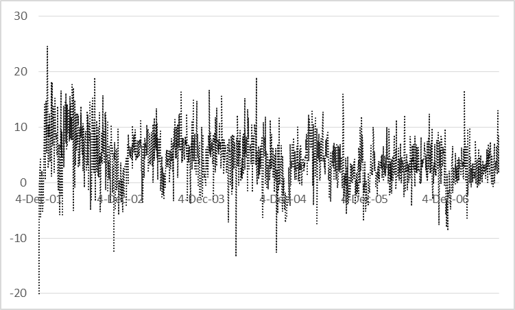
Figure 1a

Slope of LIBOR-OIS term structure, 12-month LIBOR-OIS spread less one-month LIBOR-OIS spread, December 4, 2001 to July 31, 2007. The slope is measured in basis points. Source: Bloomberg

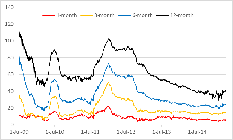
Figure 1b

Post-crisis LIBOR-OIS spread for different tenors (basis points). Source: Bloomberg

Pre-crisis it was possible to (a) calculate a zero curve from LIBOR deposit rates and swap rates, (b) construct a model of the short-term LIBOR rate, and (c) use it to calculate the value of an interest rate derivative.  In Hull and White (1994a, 1996, 2001) we develop a way this can be done using a trinomial tree. A trinomial tree is equivalent to the lattice used in the explicit finite difference method.

It is no longer appropriate to build a term structure model directly for LIBOR interest rates for two reasons. First, as already mentioned, it is no longer reasonable to treat the LIBOR rate as a proxy for the risk-free rate. Second, a single LIBOR zero curve no longer exists. LIBOR zero curves can be constructed from swap rates, but there is a different LIBOR zero curve for each tenor.

One approach to term structure modeling is to use the methods in Hull and White (1994a, 1996, 2001) to build a tree for the short-term OIS rate and assume that the LIBOR-OIS spread is deterministic. For example, if a Bermudan swap option is being valued where the tenor of the underlying swap is six months, the procedure would be as follows:

1. Construct a trinomial tree for the short-term OIS rate so that it is consistent with OIS zero rates, ensuring that nodes lie on reset dates for the underlying swap. The tree should extend to the end of the underlying swap.
2. Calculate the six-month OIS rate on each reset date of the underlying swap by rolling back through the tree.
3. Add the (deterministic) six-month LIBOR-OIS spread to determine the six-month LIBOR rate on each reset date of the underlying swap
4. Roll back through the tree to value the Bermudan swap option. The swap cash flows are determined by the six-month LIBOR rates. The Dt-OIS rates, where Dt is the length of each time step on the tree, are used to discount the cash flows back through the tree.

In Hull and White (2016) we show how the method can be extended so that the LIBOR-OIS spread is stochastic. The first two steps are the same. We then proceed as follows:

3. Choose a stochastic process for the six-month LIBOR-OIS spread. This will incorporate a function of time in the drift so that the forward LIBOR rates can be matched. At this stage, a “preliminary tree” is created where the function of time is set equal to zero.
4. Create a three-dimensional tree from the OIS tree and the preliminary spread tree assuming zero correlation between the OIS rate and the spread. The probabilities on the branches of this three-dimensional tree are the product of the probabilities on the corresponding branches of the underlying two-dimensional trees.
5. Build in correlation between the OIS rate and the spread by adjusting the probabilities on the branches of the three-dimensional tree. One way of doing this is described in Hull and White (1994b).
6. Work forward through the tree, using an iterative procedure, determining the function of time mentioned in step 3 so that forward LIBOR rates observed in the market are matched. The matching is achieved by ensuring that forward rate agreements where LIBOR forward rates are exchanged for realized LIBOR have a value of zero.

The tree is then complete and can be used to value a Bermudan swap option or other instrument.

This type of tree approach provides an alternative to Monte Carlo simulation for simultaneously modeling spreads and OIS rates. It can be regarded as an extension of the explicit finite difference method and is particularly useful when American-style derivatives are valued. It avoids the need to use techniques such as those suggested by Longstaff and Schwartz (2000) and Andersen (2000) for handling early exercise within a Monte Carlo simulation.  

References

Andersen, Leif (2000), “A Simple Approach to Pricing Bermudan Swap Options in the Multifactor LIBOR Market Model,” Journal of Computational Finance, 3, 2: 1-32.

Hull, John and Alan White (1994a), "Numerical procedures for implementing term structure models I," Journal of Derivatives, 2 (Fall), pp 7-16  

Hull, John and Alan White (1994b) "Numerical procedures for implementing term structure models II," Journal of Derivatives, Winter, pp 37-48.

Hull, John and Alan White (1996), "Using Hull-White interest rate trees," Journal of Derivatives, Vol. 3, No. 3 (Spring), pp 26-36.

Hull, John and Alan White (2001), “The General Hull-White Model and SuperCalibration,” Financial Analysts Journal, 57, 6 (Nov-Dec): 34-43.

Hull, John and Alan White (2013), “LIBOR vs. OIS: The Derivatives Discounting Dilemma” Journal of Investment Management, Vol 11, No. 3: 14-27.

Hull, John and Alan White (2016), Multicurve Modeling Using Trees” Forthcoming in Challenges in Derivatives Markets Editors: Kathrin Glau, Matthias Scherer, and Rudi Zagst, Springer Proceedings in Mathematics and Statistics.

Longstaff, Francis A. and Eduardo S. Schwartz (2001), “Valuing American Options by Monte Carlo Simulation: A Simple Least Squares Approach,” Review of Financial Studies, 14, 1:113-147.