Blog

In our last blog we discussed the different models that can be used when interest rates are low or negative and how the models can be calibrated to market data. When standard transactions such as caps, floors, and swaptions are being considered, the model being used does not have an appreciable effect on the price. This sounds counterintuitive, but is a direct result of the way models are used by practitioners. The model is nothing more than a sophisticated interpolation tool. Prices for transactions with standard strikes and times to maturity are observed in the market. Volatility parameters (if not quoted in the market) are implied from these prices and traders interpolate between the volatility parameters to determine the volatility parameters for deals with nonstandard strikes or times to maturity.

However, the model used can have a big effect on how hedging is done. For example the DV01 calculated from the shifted lognormal model will not in general be the same as the DV01 calculated from the Bachelier normal model. It might be supposed that it does not matter which model a trader uses provided:

1. The model always matches market prices, and
2. The trader hedges against all the changes that could affect the calculated price given by the model.

A Taylor Series expansion of the price in terms of all the variables that can change through time suggests that this is the case. But in practice adequately hedging the volatility parameter applicable to a particular instrument (cap or swaption) is liable to be difficult. But in practice adequately hedging the volatility parameter applicable to a particular instrument (cap or swaption) is liable to be difficult.

As explained in our previous blog, the shifted lognormal model assumes that $F+s$ follows the same lognormal process as that normally assumed for $F$ where $F$ is the relevant forward rate and $s$ is a shift. In the Bachelier normal model, the forward rate follows a normal diffusion process and future values of $F$ are normally distributed. In both models the size of the volatility parameter, $\sigma$, is different for each option strike rate and each maturity.

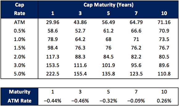
We shall illustrate the impact of the model chosen using data from March 1, 2016. Table 1 shows shows the volatilities implied from the Bachelier normal model (in basis points) and the at-the money strike rate (defined so that the cap price equals the floor price). As the table shows, the at-the-money strike rate was negative for maturities out to seven years.  The volatilities can be converted into prices using the formula given in our previous blog and shifted lognormal volatilities can then be implied. 

Table 1: Broker quoted Bachelier normal volatility parameters (in basis points) for caps. The lower panel shows the at-the-money (ATM) cap rates. 

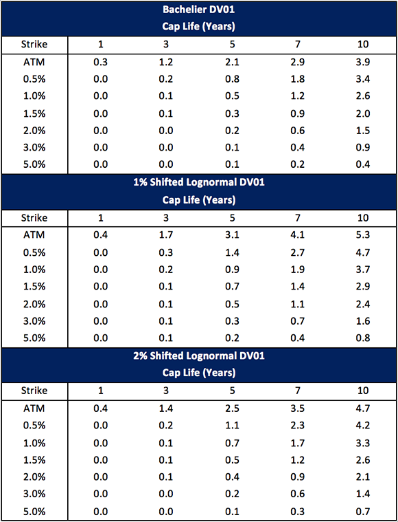
The DV01s for the shifted lognormal model and the Bachelier normal model are shown in Table 2. Two versions of the shifted lognormal model are considered. In one the shift is 1%; in the other the shift is 2%. In all cases, DV01 is calculated keeping the volatility parameter constant (as is the usual market practice).

The table shows that the Bachelier model produces DV01s that are materially smaller than those produced by the shifted lognormal model. In absolute terms the difference is largest for long maturity at-the-money options while in proportional terms the difference is largest for short maturity out-of-the-money options. Also, when the shift applied to the lognormal model is increased, the DV01s decline. Although the three models agree on the price of the cap, there are material differences in the sensitivity to interest rate changes given by the models.

A more sophisticated model sometimes used by traders is the SABR model. As explained in our previous blog this has a number of parameters $\left( \sigma, \beta, \xi, \mbox{and }\rho \right)$ and can provide a good fit to the volatility smile for options with a particular maturity. It also reflects smile dynamics reasonably well. However, the volatility parameters are different for different option maturities. When choosing the volatility parameters to fit all options with a particular maturity $\sigma$ and $\beta$ have similar effects. As a result, users generally select a value for $\beta$ such as $\beta$ = 0.5 and then find the values for the other three parameters that best fit the observed prices. When a price is to be calculated the SABR parameters calibrated for standard option maturities are interpolated based on option maturity.

Table 2: Change in the cap price measured in basis points as a result of a one basis point increase in the zero curve for three different models.

The change in the expected initial volatility of the forward rate given the change in the forward rate is

\[ \mathbb{E}\left( d\sigma | dF \right) = \xi \rho dF /F^\beta \]

This expected change in the volatility as a result of a change in the forward rate then has an effect on the expected DV01[1] calculated as:

\[ \mathbb{E}\left( DV01 \right) = f_{SLN} \left( F_0 + \Delta F, \sigma_{imp} \left( F_0 + \Delta F, \sigma_0 + \xi \rho \Delta F/F^\beta \right) \right) - f_{SLN}\left(F_0, \sigma_{imp} \left( F_0, \sigma_0 \right) \right)\]

where $ f_{SLN} \left( F, \sigma \right)$ the value of an option given by the shifted lognormal model when the forward rate is $F$ and the volatility is $\sigma$, and $\sigma_{imp} \left(F, \sigma_0 \right)$ is the SABR implied volatility when the forward rate is $F$ and the initial volatility of the forward rate is $\sigma_0$. $F_0$ is the forward rate based on the initial zero curve and $\Delta F$ is the change in the forward rate as a result of a 1 basis point increase in the continuously compounded zero curve. This expected DV01 is calculated for each caplet; the DV01 of the cap is the sum of these caplet DV01s.

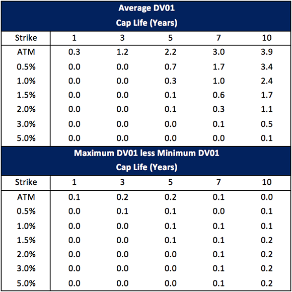
We considered four versions of the SABR model: $\beta$= 0.5 shift = 1%, $\beta$= 0.5 shift = 2%, $\beta$= 1.0 shift = 1%, and $\beta$= 1.0 shift= 2%. Each of these models was calibrated to the options in Table 1 in the following way. For a particular value of $\sigma$, $\xi$ and $\rho$ each of the option prices for a particular maturity was calculated using the model version. These prices were used to imply a Bachelier implied volatility. The values of $\sigma$, $\xi$ and $\rho$ were then chosen to minimize the sum of the squared difference between the implied Bachelier volatilities and the volatilities in Table 1. This resulted in 5 sets of parameters, one for each option maturity, for each version of the model. For three of the model versions the models fit the data well; the root mean squared difference in the Bachelier volatilities for each option maturity is less than one basis point. Each of these three model versions also produce similar values for the DV01. The $\beta$= 1.0 shift = 1%, version does not fit the data well and produces DV01s that are very different from the other three versions. As a result we did not include this version in our analysis.

Table 3 reports the average DV01 calculated by the three SABR models included in our analysis as well as the difference between the maximum DV01 and the minimum DV01 calculated by the three models for each option maturity and each strike. The range of DV01s for any maturity and strike is never larger than 0.2 basis points. This is an interesting result. It shows that the models agree fairly well on the DV01 provided they are calibrated to the same term structure and volatility smile

The Bachelier and SABR DV01s also agree quite closely. The root mean square difference between Bachelier and SABR DV01s is 0.18 bp for all options and 0.24 bp for options with lives greater than 5 years. The root mean square difference between shifted lognormal (2% shift) and SABR DV01s is larger: 0.49 bp for all options and 0.66 bp for options with lives greater than 5 years. The differences for the 1% shifted lognormal model are even larger.

Table 3: Average DV01 measured in basis points and the difference between the highest and lowest DV01s calculated for each option using three versions of the SABR model: $\beta$ = 0.5 shift = 1%, $\beta$ = 0.5 shift = 2%, and $\beta$=1.0 shift = 2%.