

In 2013, Nick DeGuillaume, Riccardo Rebonato and Andrei Pogudin published some interesting research on the volatility of interest rates.[1] They looked at different interest rates in different countries over different time periods. They concluded that there is a “universal relationship”: the short rate exhibits approximate lognormal behavior when the rate is low or high. For intermediate values of the rate, the behavior is approximately normal. The process derived from historical data by Deguillaume et al is
$$dr = \dots+ \sigma ( r ) dz$$
where
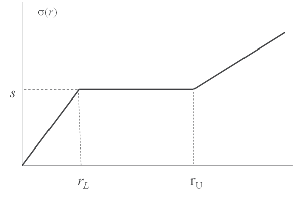
$$\sigma(r) = \begin{cases} s r / r_L & \mbox{when} \quad r \leq r_L \\ s& \mbox{when} \quad r_L r \le r_U \\ s + \beta \left( r- r_u \right) & \mbox{when} \quad r > r_U\end{cases}$$
This function is illustrated in Figure 1.
Typically $r_L$ is about 1.5% and $r_U$ is about 6%. Thus Deguillaume et al contended that rates tended to be lognormal when they are less than 1.5%, normal when they are between 1.5% and 6% and lognormal above 6%. Their results were based on historical data. They were therefore estimating the process followed by rates in the real world. However, Girsanov’s theorem tells us that the volatility of an interest rate (or any other variable) should be the same in both the real world and the risk-neutral world. If Deguillaume et al’s results are correct we know the volatility of the short rate in the risk-neutral world and can use it to value derivatives.
In Hull and White (2015) we decided to test this out by finding which piecewise linear representation of the short rate standard deviation, similar to that shown in Figure 1, best fit cap data. We first developed a procedure for rounding the corners of the volatility function so that the function was both continuous and differentiable.
Suppose that the best fit volatility function (not necessarily the one in Figure 1) is $G(r)$. We then define a variable $x$ which is a function of $r$ as
$$x = f(r) = \int \frac{1}{G(r)} dr$$
Figure 1
Deguillaume et al’s result for the variability of the short rate as a function of the short rate
 In this case the process for $x$ is
$$dx = \dots dt+ dz$$
If we assume that the drift of x in a risk-neutral world is $\theta (t) - ax$ then the process for $x$ is
$$dx = \left[ \theta (t) -ax \right] dt + dz$$
This would allow us to use the tree-building procedures we developed in Hull and White (1994, 1996, and 2001) for valuing derivatives. The function $\theta (t)$ is chosen so that the process provides an exact fit to the current term structure.
Although this approach is theoretically acceptable we found that when $x$ follows this generalized mean reverting process the drift of $r$ may be unreasonable. We therefore developed a way of modifying our tree-building procedure so that a range of different drifts for $r$ could be assumed. A natural assumption is that $r$ (not $x$) followed a generalized mean-reverting process so that:
$$dr = \left[ \theta (t) -ar \right] dt + G(r)dz$$
Again, the function $\theta (t)$ is chosen so that the process provides an exact fit to the current term structure.
We first assumed that $G(r)$ in equation (1) was a piecewise linear function defined by corner points at 1%, 2%, 3%, 4%, 5%, 6%, and 10%. We calibrated the model as closely as possible to the prices of caps observed on December 2, 2013. Our goodness-of fit measure was
$$\sum_{i=1}^N\frac{\left(U_i - V_i \right)^2}{U_i}$$
where $N$ is the number of different caps used and $U_{i}$ and $V_{i}$ are the market price and model price of the $i-$th cap. An optimizer was used to find the corner points that minimized the objective function.
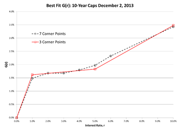
The resulting $G(r)$ is shown in Figure 2. Because of the large number of degrees of freedom in the calibration, the fit to the market prices is very good. Unfortunately, the type of high dimensional optimization involved in determining the best fit $G(r)$ function with 7 corner points is both time consuming and difficult. However, an examination of the $G(r)$ function illustrated in Figure 2 shows that a simpler functional form may be acceptable. To explore this possibility we recalibrated the model using a $G(r)$ with only three corner points: 1%, 5% and 10%. The result of this is also shown in Figure 2.
Figure 2
The best-fit $G(r)$ function calibrated to 10-year cap prices from December 2, 2013. Two different functional forms are used. In the first case $G(r)$ is a piecewise linear function defined by 7 corner points. In the second case $G(r)$ is defined by 3 corner points.
As another test we calibrated the model to cap prices observed between 2004 and 2013. Market data for caps observed on the last trading day of March in each year were used. To minimize the effect on the calibration of very high and very low strike options the cap quotes used for a particular maturity were those where the cap rate was within 1.5 standard deviations of the at-the-money strike price.[2] Because of this filtering the short-dated caps that are included in the calibration generally have fairly low strike prices. We were concerned that this might affect to calibration process, particularly the portion of the $G(r)$ function that applies to high rates. As a result we divided the cap data into two groups: caps with maturities between 1 and 10 years and caps with maturities between 10 and 30 years. The $G(r)$ function for each year was estimated for these two groups separately. In each calibration, the model was fitted to about 50 caps with different strikes and maturities.
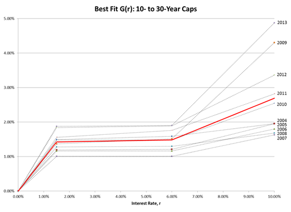
The choice of the corner points in the parameterization of $G(r)$ was determined by experimentation. We first tried the corner points used when calibrating to the December 2013 data, 1% and 5%. We then tried 2% and 6% and ultimately decided to use 1.5% and 6% on the grounds that the goodness of fit for these corner points was slightly better on average than for the alternatives. The results are illustrated in Figures 3 and 4. In every year the $G(r)$ function has the same shape as the Deguillaume et al function. Further, there is a high degree of similarity between the results for calibration to short-term caps and calibration to long-term caps in each year. Most of the deviation is observed in the value of $G(r)$ for high values of $r$ where the short term caps provide little information.
The volatility structure implied by cap prices is similar to that observed in the real world. The structures calibrated from cap prices provide a measure of the volatility structure at a point in time. As the results show, this changes from year to year and probably from day to day. Since we cannot observe the real world volatility structure over short periods of time the best we can say is that these results are consistent with Girsanov’s theorem. Overall, our results are supportive of the conjecture that the volatility function used (implicitly or explicitly) by market participants when pricing interest rate caps is similar to the volatility function derived by Deguillaume et al. What is more, this was true even before the Deguillaume et al research was first available as a working paper.
Since 2013 rates in Europe and elsewhere have dipped below zero. Currently, the Euro LIBOR term structure is below zero for maturities up to about 7 years. This means that the lognormal structure for rate volatilities for low rates found by us and Deguillaume et al will have to be modified. Dealing with negative rates will be the subject of a future blog.
Figure 3
The best-fit $G(r)$ function calibrated to 1- to 10-year cap prices from 2004 to 2013. The solid line shows the average of the ten $G(r)$ functions.
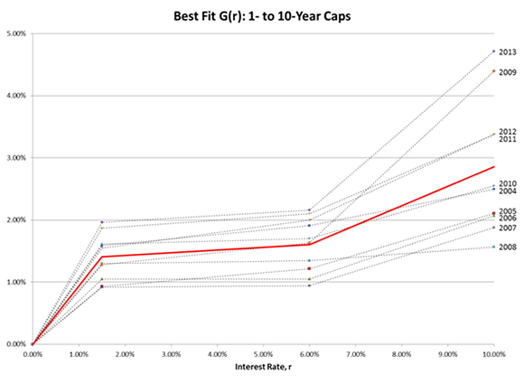
Figure 4
The best-fit $G(r)$ function calibrated to 10- to 30-year cap prices from 2004 to 2013. The solid line shows the average of the ten $G(r)$ functions
[1] See N. DeGuillaume, R. Rebonato, and A. Pogudin (2013)
[2] The standard deviation was the average cap volatility for the maturity being considered multiplied by the square-root of the cap maturity.
References
DeGuillaume N., R. Rebonato, and A. Pogudin, “The Nature of the Dependence of the Magnitude of Rate Moves on the Level of Rates: A Universal Relationship,” Quantitative Finance, 13, 3 (2103): 351-367.
Hull, J. and A. White, "Numerical procedures for implementing term structure models I," Journal of Derivatives, 2 (Fall, 1994)): 7-16
Hull, J. and A. White, "Using Hull-White interest rate trees," Journal of Derivatives, Vol. 3, No. 3 (Spring, 1996): 26-36.
Hull, J. and A. White, “The General Hull-White Model and SuperCalibration,” Financial Analysts Journal, 57, 6, (Nov-Dec 2001): 34-43
Hull, J. and A. White, “A Generalized procedure for Building Trees for the Short Rate and its Application to Determining Market Implied Volatility Functions,” Quantitative Finance, 15, 3 (2015): 443-454.