Dominic Brecher, a Quantitative Analyst at FINCAD, has a PhD in high-energy theoretical physics from the University of Cambridge. In addition, he has conducted postdoctoral research in String Theory at the Universities of Durham and British Columbia. With several papers published in the Journal of High Energy Physics, Nuclear Physics and Physical Review, he has recently brought his extensive research experience in physics to the world of financial engineering. Combining theoretical requirements and industry practice, Dominic designs derivative pricing models and explores their consequences in the financial markets. In this article, he explains what he has learned about the theory of local volatility in option pricing, and discusses its practical implementation in FINCAD Analytics Suite and FINCAD Analytics Suite Developer.

» To download the latest trial version of FINCAD Analytics Suite, contact a FINCAD Representative.

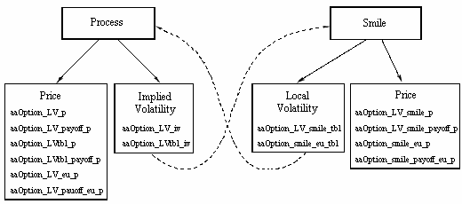
This will include functions to price European and American options, option strategies, portfolios of options, and options with arbitrary piecewise linear payoffs, from the smile as described in this article. All numerical pricing is done through the no-arbitrage PDE. Other functions start instead with a given local volatility process defined either by standard parameterizations (such as the CEV, normal and shifted lognormal processes), or a user-defined data table. These functions also price European and American options, option strategies, portfolios of options, and options with arbitrary piecewise linear payoffs, and can be used to back out the corresponding implied volatility smile. Using a combination of the two sets of functions, further issues such as the corresponding implied volatility smile. Using a combination of the two sets of functions, further issues such as the smile dynamics can be analyzed. Starting with either a given local volatility function, or with a given implied volatility smile, the interplay between these functions is shown below.

What's Right and Wrong with Black-Scholes?

Despite its many deficiencies, the Black-Scholes model of option pricing [1] remains widely used, some 30 years after its inception. It is still the first model that both quants and traders reach for when given a deal to price. Quants like it because it provides a theoretically consistent framework to price options in almost any asset class, given some (possibly dubious) assumptions. Traders like it because of the tractability of the Black-Scholes formula for option prices, and because it is easily tweaked to account for their intuition about the market.

The Black-Scholes formula allows the fair price of a European option to be determined, given various observables - current asset price, strike price, time till maturity, risk-free rate and dividend yield - and a single unobservable constant - the volatility, σ, of the underlying asset price. Historical volatility is easily determined, though this is not necessarily a good guide as to how the future asset price will change. One is ultimately left with making a (more or less) educated guess as to the magnitude of σ, the likely average future volatility.

Volatility as a Unit of Currency

Traders have turned this drawback of the Black-Scholes model into a useful feature, by quoting European option prices not in terms of their dollar value, but in terms of the equivalent implied volatility. This is the value of σ which must be used in the Black-Scholes formula to give back the market price of that specific option. If the market price of some call option is C, then the implied volatility (a function of asset price S, strike K and maturity T) is defined through the relationship

C(S,K,T) = C_BS(S,K, σ(S,K, T), T), (1)

where C_BS is the Black-Scholes price of the option.

It is thus always possible to determine the market's view of the future volatility of some asset from quotes for options written on that asset: it is just the implied volatility at which the options trade.

Using volatility as a unit of currency in this way is only possible due to some underlying properties of the Black-Scholes framework. Most importantly, the price of an option is a monotonically increasing function of volatility. If option prices were multi-valued functions of volatility then there would be no useful price ↔ volatility correspondence.

The ability to quote option prices in terms of a constant volatility is partly why the Black-Scholes model is still so widely used in the market. However, it makes the most important deficiency of the Black-Scholes framework transparent: the market-observed volatility is simply not a constant.

The Volatility Smile

At least since the crash of 1987, the market-observed implied volatilities of European equity options have exhibited a distinct "skew" structure. Deep out-of-the-money puts generally trade at higher implied volatilities than out-of-themoney calls. An example - for options on the S&P 500 index - is shown in Figure 1. One reason is that this reflects the market's appetite for insurance against stock prices falling. Options on interest rates - caps, floors, swaptions - also generally exhibit such a volatility skew. Other options exhibit a volatility "smile", in which both deep out-of-the-money calls and puts trade at higher implied volatilities than their at-the-money counterparts.

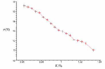
Figure 1. A volatility skew: implied volatilities, as of July 19, 2006, for European options on the S&P 500 index, expiring August 19, 2006. The mid-price implied volatilities of call and put options have been averaged and plotted against the "moneyness" K/S₀ where S₀ – 1258.05 is the current underlying price.

We refer to the variation of implied volatility with strike price as the "volatility smile" despite the fact that a skew, frown, smirk or other such structures are often seen in the market. The implied volatility of traded options also varies with the option maturity - the volatility term structure - and so one often talks of an implied volatility surface: σ = σ(K, T) is a function of two variables. Points on the implied volatility surface for options on the S&P 500 index are shown in Figure 2.

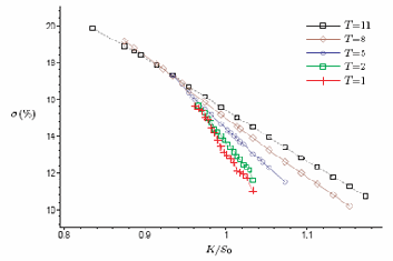
Figure 2. Points on a volatility surface: implied volatilities, as of July 19th, 2006, for European options on the S&P 500 index, expiring at various times (T is in months in the key). The underlying price is 1258.05, and the mid-price implied volatilities of call and put options have been averaged.

It is easy to modify the Black-Scholes framework to deal with a volatility term structure, but the model simply does not allow for volatilities to vary with strike price. Once one recognizes this it becomes clear that, in the words of Rebonato, implied volatility is really only the "... wrong number to put in the wrong formula to obtain the right price of plain vanilla options" [2].

Beyond Black-Scholes

Arguably the most important problem in the theory of option pricing is how to take account of the volatility smile. This is far from a purely academic exercise. Given the skew shown in Figure 1, for example, what would be the correct volatility to use to price a European option struck at 1295? Whilst fairly easy to answer (one would use some form of interpolation on the volatility smile), it is less clear what volatility to use to price the corresponding American option, and much, much less clear what value to use to price an exotic contract, say a knock-in barrier option.

The real motivation for considering the effects of the volatility smile in option pricing is precisely this: to calibrate one's pricing of exotic, or even just American, options to the market-observed prices of European plain vanillas. Various models have been developed over the years to go beyond Black-Scholes in this way. They include:

• Jump-diffusion models, introduced by Merton [3];
• Stochastic volatility models, introduced by Hull and White [4]. The Heston [5] and SABR [6] models are two of the most popular;
• Local volatility models, introduced by Dupire [7], Derman & Kani [8] and Rubenstein [9];
• Models in which the underlying stochastic process is a mixture of lognormal distributions, introduced by Brigo and Mercurio [10].

We will be reviewing local volatility models¹ in this article.

Volatility and Stochastic Processes

The constant volatility of the Black-Scholes framework corresponds to the assumption that the underlying asset follows a lognormal stochastic process in the risk-neutral measure

dS = rS dt + σS dW,

where dW is a Brownian motion, and we will throughout assume a constant risk-free rate r and no dividends. The return on the asset over some time period T is thus normally distributed with a standard deviation of σ √T. This is the basic property which makes the model analytically tractable.

As the name suggests, local volatility can be thought of as taking the constant volatility, σ, and replacing it with a function which depends locally both on time and on the value of the underlying asset: ∑=∑(S, t). The lognormal property is thus no longer true within the local volatility framework. Rather the goal is to determine the correct underlying process from the market-observed smile, by determining the correct local volatility function. Note that the implied volatility σ(K, T) is a function of strike and maturity whereas the local volatility ∑(S, t) is a function of asset price and time.

With this notation, the underlying stochastic process in a local volatility model is²

dS = rS dt + ∑(S, t)S dW (2)

Using standard arguments [11], the corresponding no-arbitrage partial differential equation (PDE) for the price, V , of an option written on the underlying asset is

This is just the Black-Scholes equation, but with the constant volatility replaced by a general function ∑(S, t). Our approach will be to determine this function from the implied volatility smile, then to use standard numerical techniques to solve the PDE(3).

Dupire's Equation

The transition probability function3 associated with the stochastic process (2) satisfies both the backward (Kolmogorov) and forward (Fokker-Planck) equations. The noarbitrage equation (3) is essentially the backward equation. As shown by Dupire [7] (see also [8] and [12]), the local volatility function can in principle be determined from the forward equation. From the latter, one can derive

Both equations (3) and (4) apply in complete generality, to any option written on the asset S. The local volatility function can now be derived by specializing to European plain vanillas, say call options with prices C. Applying equation (4) to a complete set of such options (for all strikes and maturities) and upon re-arranging, we get Dupire's equation

Given the market-observed prices of plain vanillas, this equation in principle determines the local volatility at time t = T when the stock price is equal to S = K. But only in principle, since one needs a complete set of option prices to fully determine the local volatility function; and one only has access to a finite set of such prices. One might wonder whether the right-hand side of equation (5) is always positive. Indeed it is: no-arbitrage arguments guarantee it [12], although in practice interpolation and/or extrapolation issues will often lead to negative values of ∑².

In addition to this, numerical effects for deep out-of-the-money options, when the denominator⁴ of equation (5) tends to zero, lead to badly behaved local volatility functions - the numerator must tend to zero at the same rate in order that the local volatility function remain finite. For this reason, it is often preferable to rewrite equation (5) directly in terms of implied volatilities rather than option prices.

From Implied to Local Volatility Directly

The implied volatility of an option with price C(S,K,T) is defined through the Black-Scholes formula as in equation (1). The derivatives of the call price in equation (5) can thus be computed through the chain rule, and substituting for these leads to the following result [12, 13]:

and t₀ and S₀ are respectively the "market" date, on which the volatility smile is observed, and the asset price on that date.

Equation (6) is the basic result. Not only is it difficult to analyze analytically, but it is also not particularly wellbehaved numerically. Small changes in the implied volatility lead to large changes in the local volatility, and in fairly unpredictable ways.

However, equation (6) can in principle be used to determine the local volatility function from the market-observed smile. This can then be used through the PDE (3) to give option prices which are calibrated to the European plain vanillas seen in the market.

Pricing Techniques

To price a European option from the smile, one only needs to interpolate from the market-observed implied volatilities to the strike and maturity of the option in question. The price will only be as good as one's interpolation scheme, and research continues into the pros and cons of various methods (see, e.g., [14]). To price an American option, or anything at all exotic, we need to use the local volatility function in conjunction with a numerical method to solve equation (3). The interpolation from the implied volatility surface to various strikes and/or option maturities is just the first step. We then have to compute the local volatility through equation (6) at each relevant point in (S, t) space.

Implied Trees

The original work of Dupire [7], Derman & Kani [8] and Rubenstein [9] all used binomial or trinomial trees to encode the local volatility function. To construct the tree, one ensures that, at each (S, t) node, an option with (K = S, T = t), is priced correctly.

The procedure is notoriously unstable. Even after just a few time-steps, negative branching probabilities are encountered which one has to re-set by hand, although the problem is somewhat better if one uses an approach based on forward rather than spot prices [15]. Moreover, the local volatility function which one can back out from such an implied tree does not have particularly intuitive properties, as discussed at length in [2].

In addition to this, the tree-based approach would have all the usual problems when applied, for example, to more exotic instruments such as barrier options. For these reasons, a PDE approach to option pricing is preferred.

PDEs

Given a local volatility function, it is easy to apply standard numerical techniques to solve the no-arbitrage PDE (3) for option prices. We use the Crank-Nicolson scheme for well-documented reasons [13]. The application of local volatility to such finite difference methods was first discussed in [12].

We will not review the Crank-Nicolson method in any detail here. Suffice it to say that we have set up a grid of points in (S, t) space, and that the derivatives in equation (3) have been approximated using finite differences. The grid points are labeled by i and j as S_min ≤ S_i ≤ S_max and t₀ ≤ t_j ≤ T₀ where the option maturity is denoted by TB0B. The next step is to determine the value of ∑ at every grid point (i, j). As for the implied trees discussed above, we need to be able to reproduce option prices for all values of K = S_i and T = t_j in our grid.

The procedure used in [12] to determine the discrete local volatility function is numerically involved and somewhat unstable. For these reasons, we prefer to work with the result (6), which relates the local volatility function directly to the implied volatility smile. A simple finite difference approximation for the derivatives in equation (6), along the lines discussed in [2], is the simplest way to generate the discrete local volatility function, and seems to give results at least as good as any other procedure.

Whichever approach one takes, the problem is ultimately how to interpolate and/or extrapolate the observed implied volatility surface. Given a finite set of data points, how do we generate implied volatilities for all values of K = S_i and T = t_j? This is a real problem since the results depend very sensitively on the interpolation method.

Thankfully such effects, as long as they are localized, do not lead to large differences in option prices. In that sense, the actual behaviour of the local volatility function is not too relevant to option pricing.

Interpolation of the Implied Volatility Surface

Given a set of implied volatilities as in Figure 2, there are various interpolation methods one might use. Both parametric and non-parametric methods have been discussed in the literature, a selection of these including:

• Standard bi-linear or bi-cubic splines;
• Entropy minimization techniques [16];
• Smoothing techniques such as Nadaraya-Watson smoothing [17];
• Dimension reduction techniques such as Principle Component Analysis [14]

Each method has its benefits and drawbacks. The only certain thing is that the local volatility function depends very sensitively on the implied volatility σ and its derivatives, in particular on the derivatives of σ with respect to the strike price K.

This dependence can be made less sensitive by using smoothing techniques. A simple such technique - using smooth cubic splines - was discussed originally in the context of probability density functions [18], and applied to the implied volatility surface in [19]. The latter work also showed how to apply no-arbitrage constraints to the procedure in a relatively straightforward way.

Thin Plate Splines

The smoothing technique is applied in the strike direction only. In the context of probability density functions [18], one is after all only interested in the implied volatility as a function of strike price, for options of a single maturity. For the grid-based option pricing methods at hand, however, we need the implied volatility as a function of strike price, for all maturities T = t_j in our grid. We will thus construct a smooth cubic spline in strike space at each timestep in our grid. To generate the implied volatilities to be smoothed at each time-step, we first need to construct a pre-smoothed surface. This can be done using a bi-linear or bi-cubic spline, but a better method is to use a thinplate spline [19]. One may, for instance, only have data for a few different strikes at each maturity, and these strikes may differ across maturities. Such a data set would not be well-suited to bi-linear or bi-cubic interpolation. A thin plate spline is the natural two-dimensional generalization of the cubic spline, in that it is the surface of minimal curvature through a given set of two-dimensional data points. Denoting these points by , the objective function is given by

where The coefficients a_i, b_i can be found through straightforward linear algebra [20]. In our case, the dimensionless coordinates (K/S₀, T/T₀) should be used.

Our procedure is thus as follows:

• Construct a thin-plate spline through the given set of implied volatility data points. This is our presmoothed surface.
• Starting from the final time-step in the grid, evaluate the thin-plate spline at that value of T = t_j and at some representative number of strikes (say 20), between K = S_min and K = S_max.
• Construct a smooth cubic spline through these points (see below).
• Evaluate the resulting cubic function at all values of K = S_i for that time-step.
• Compute the derivatives of the implied volatility in equation (6) using standard finite difference
  approximations. (The ∂/∂T term needs the smooth spline for at least two adjacent time-steps.)
• Put everything together as in equation (6) to compute the value of ∑(S_i, t_j) at each grid point S_i at that time-step.
• Use these values in the Crank-Nicolson scheme to solve for option prices, and then move to the next time-step.

Smooth Cubic Splines

The smooth cubic splines are easy to construct. The objective function is piecewise cubic in K:

where i runs over the points at which the thin-plate spline is evaluated by each timestep (i = 1, . . . 19 in the above). The usual continuity conditions hold on g(K) and its first two derivatives. A smooth cubic spline is then constructed as the minimizer ^∧g of the penalized sum of squares⁵

the penalty function being equal to the integrated (squared) curvature. The constant λ is the smoothing parameter, controlling the weight of the penalty function. Using the moneyness coordinate K/SB0B in equation (7) ensures that λ is dimensionless. For λ ≥ 0, there is a unique minimum; and there exists a simple algorithm involving only some elementary linear algebra to compute it [20]. For λ = 0, one recovers the standard natural cubic spline, going through all data points. For λ → ∞, one instead generates a least-squares fit. Figure 3 shows an example of a smooth cubic spline through the volatility smile of figure 1, for options on the S&P 500 index.

There are various criteria which can be used to determine what is the "best" value of λ [20], although not all of these produce good results in the financial context [21]. At any rate, the smoothing procedure acts to reduce the (absolute value of the) curvature of the implied volatility surface in the strike direction. The net effect is to make the local volatility function dramatically smoother. On the other hand the resulting spline(s) will no longer go through all (if any) of the original implied volatility data points. One might object that this takes us away from the original market data, but perhaps this does not matter too much. After all, there is always some room for manoeuvre due to the bid-ask spread. Indeed, for deep out-of-the-money options this spread can be very large when converted to volatility space.

An Example: Pricing an Option with Local Volatility

To make the above discussion more explicit, consider pricing an at-the-money European call option on the S&P 500 index, calibrated to the implied volatility data of Figure 2, and expiring in T₀= 11 months. For definiteness, we take the continuously compounded risk-free rate and dividend yield to be, respectively, 6% and 2%. To price the option, we set up a grid in (S, t) space with 40 steps in each direction. We start with the smoothing parameter λ = 0, an naively apply the procedure given in the previous section. The implied volatility surface at points in our grid is shown in Figure 4. An immediate problem should be apparent - the implied volatility is negative for large regions of the grid!

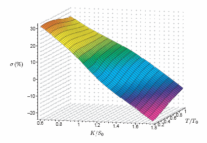
Figure 4. The implied volatility surface in our grid with λ = 0

Ignoring this problem for the time being, the local volatility function used in our grid is shown in Figure 5. Although it cannot be seen from the figure, for some parts of our grid ∑squared also turns out to be negative! (We have set ∑ = 0 in those regions.) Apart from this (nevertheless important) fact, the local volatility function looks fairly well behaved.

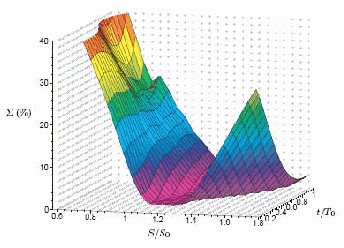
Figure 5. The local volatility function in our grid. Although hard to see from this plot, since
Σ² 0 in some regions, we have set Σ = 0 anywhere this occurs.

The numerical price and first few risk statistics of the European option, for various numbers of steps in (S, t) space are given by:

	40 x 40 steps	100 x 100 steps	200 x 200 steps
price	94.0553	94.3058	94.3133
Δ	0.4480	0.4455	0.4455
Γ	0.00219	0.00218	0.00204
Θ	-0.1190	-0.1181	-0.1185

The expected Black-Scholes price is 94.7719, found by reading off the value of σ = 15.3996% from the (S = 1258.05, t = 11months) grid point. The Greeks are not comparable between models, whereas the price should be (in the continuous limit).

Negative values ∑² of are obviously bad but, in the case at hand, they do not have much affect on the option prices. The regions in which ∑² 0 are fairly localized, and the values are not too negative. In other cases, ∑² 0 in large parts of the grid which leads to non-sensical option prices, since it is a signal of arbitrage opportunities.

Extrapolation of the Implied Volatility Surface

As we found above, extrapolation of the implied volatility surface to the boundaries of our grid can lead to negative values of σ. The thin plate spline we construct through the original implied volatility data points asymptotes to a linear function (in (K,T) space), which will fairly easily give rise to such behaviour. To avoid this, we need to extrapolate in a more sensible way.

Given an implied volatility smile, extrapolation to constant values of σ at large and small strikes has the effect of pasting lognormal tails onto the probability density function of the asset price. Since liquid market data for deep out-of-the-money options is anyway hard to come by, we choose this extrapolation procedure in our numerical scheme.

A simple extrapolation to constant values outside of the range of implied volatility data will lead to discontinuities in ∂σ/∂K which would in turn lead to spikes in the local volatility function. To avoid this, we instead add points to the implied volatility data out to the boundaries of our grid, before constructing the thin-plate spline. At each option maturity in the data shown in figure 2, we add extra points at constant values of σ, out to K = S_min and S_max. If need be, we also extrapolate in the T direction in a similar manner.

Having added points in this way, we then construct the thin plate spline and proceed as above. Again with the smoothing parameter λ = 0, the resulting implied volatility surface for our grid is shown in figure 6. Note that it is now everywhere positive. The price we pay is that it is considerably less smooth. In particular, our extrapolation procedure leads to a certain amount of overshoot; but there are no discontinuities in ∂σ/∂K.

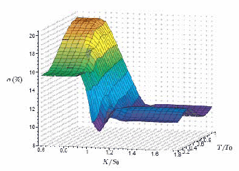
Figure 6. The implied volatility surface in our grid after the extrapolation procedure described in the text.

Although the extrapolation procedure should stop the implied volatility from becoming negative, it may still allow regions in the grid for which ∑² 0. To avoid this latter behaviour we further introduce a cut-off at, say, 2%, and demand that ∑² > = 2% everywhere. (For the case at hand, this cut-off is not necessary, but for other implied volatility data it certainly is.) At any rate, the improved local volatility function in our grid is shown in figure 7. Both plots in figures 6 and 7 are obtained using the FINCAD function aaOption LV smile tbl, available as of the Version 10 release of FINCAD Analytics Suite and FINCAD Analytics Suite Developer.

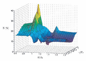
Figure 7. The local volatility function in our grid after the extrapolation procedure described in the grid. Note the differences with that in figure 5.

With this local volatility function, the price and risk statistics of our European option are

	40 x 40 steps	100 x 100 steps	200 x 200 steps
price	94.2248	94.6228	94.7043
Δ	0.4916	0.4872	0.4866
Γ	0.00190	0.00186	0.00187
Θ	-0.1246	-0.1218	-0.1231

where now σ = 15.4061% at the (S = 1258.05, t = 11months) grid point, giving a Black-Scholes price of 94.8011. These results are generated by the FINCAD function aaOption LV smile p, also available as of the Version 10 release of FINCAD Analytics Suite and FINCAD Analytics Suite Developer. Although changing the local volatility function drastically, the extrapolation procedure has not made such a big difference to these numbers.

Adding Some Smoothing

With no smoothing, the local volatility function has some rather large spikes as can be seen from Figure 7. The function is better behaved once we introduce some smoothing into the interpolation of the implied volatility surface. Setting λ= 10^-3 gives an implied volatility surface as in Figure 8.

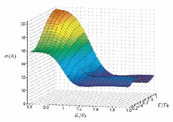
Figure 8. The implied volatility surface in our grid after the extrapolation procedure described in the text, with λ – 10^–9

The corresponding local volatility function is shown in Figure 9, both plots obtained from the FINCAD Analytics Suite function aaOption_LV_smile_tbl. As expected, the smoothing procedure gives rise to a much better behaved function. Higher values of λ would smooth out the function even more.

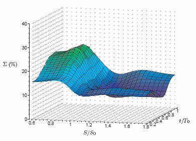
Figure 9. The local volatilty function in our grid after the extrapolation procedure described in the grid, with λ = 10^–3. Note the better behaviour as compared to the non-smoothed function in figure 7.

With the local volatility function as in Figure 9, the price and risk statistics of our European option, using the FINCAD Analytics Suite function aaOption_LV_smile_p, are:

	40 x 40 steps	100 x 100 steps	200 x 200 steps
price	94.1935	94.6149	94.7165
Δ	0.5322	0.5313	0.5308
Γ	0.00217	0.00217	0.00216
Θ	-0.1370	-0.1358	-0.1363

where σ = 15.4036% at the (S = 1258.05, t = 11months) grid point, giving the Black-Scholes price of 94.7898. It is perhaps surprising how little difference the smoothing parameter - and so the precise form of the local volatility function - makes to these numbers.

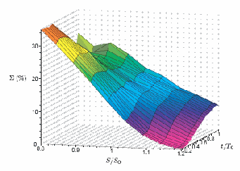
Figure 10. The local volatility function in the at-the-money region of the grid, with no extrapolation and λ = 0.

Conclusions

Rebonato has discussed general features of the local volatility function for different implied volatility surfaces [2]. For those inputs, we find similar behaviour in the "atthe-money region" of the grid. Outside of that region, however, the local volatility function can be quite badly behaved due mainly to extrapolation effects: extrapolation to constant values of σ will ultimately lead to curvature in the implied volatility surface, which in turn produces spikes in the local volatility function. On the other hand, these tend to occur in regions of the grid which are deeply in- or out-ofthe- money. Although not necessarily true for more exotic structures, the precise form of the local volatility function in many cases seems to have little impact on plain vanilla European and American option prices.

The three local volatility functions in figures 5, 7 and 9 presumably give such similar option prices because the implied volatility surfaces are similar in the at-the-money region of the grid (roughly 0.8S₀ . S_i . 1.2S₀, covering the original data of Figure 2). The corresponding local volatility functions in this region are shown in figures 10, 11 and 12, the behaviour in the three cases being qualitatively similar. The relevant region of the surface widens as it increases (see figure 2). For example, at t = 0, the only relevant value of Σ is at S = S₀

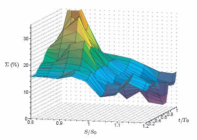
Figure 11. The local volatility function in the at-the-money region of the grid, after the extrapolation procedure, and with λ = 0.

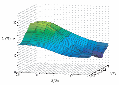
Figure 12. The local volatility function in the at-the-money region of the grid, after the extrapolation procedure, and with λ = 10^—3.

Mathematically, computing the local volatility function from the implied volatility surface is an inverse problem which is not "well-posed" [2]. Certainly, differences in the extrapolation procedure lead to large differences in the resulting local volatility function. That said, the extrapolation is to deep in- or out-of-the-money regions of the grid and the prices of plain vanilla options seem fairly insensitive to these regions. One can experiment with enforcing different extrapolation methods simply by adding extra points to the original implied volatility data; the local volatility function in the region shown in figures 10, 11 and 12 does not change much from case to case. All these issues can be explored in FINCAD Analytics Suite and FINCAD Analytics Suite Developer.

_________
Footnotes
¹Sometimes called deterministic volatility models.
²The factor of S is sometimes absorbed into the definition of the local volatility function. In our conventions, Σ has the same dimensions as σ, namely 1/√time.
³This is the probability _(S"_t"t, S_t) that the asset price equals S' at time t'given its value of S_t at time t.
⁴The denominator of equation (5) is proportional to the probability density function of the under-lying asset, so asymptotes to zero for out-of-the-money options.
⁵In [18], mainly to minimize the effect of deep out-of-the-money options, the smoothing was done in call option _ space rather than K space; and the data points were weighted by the relevant values of the options' vega. This procedure is numerically impractical to perform in a grid-based pricing method.

References

[1] Black, F. and Scholes, M. (1973) "The Pricing of Options and Corporate Liabilities,"Journal of Political Economy 81 (3), 637-659.

[2] Rebonato, R. (2004) Volatility and Correlation: the Perfect Hedger and the Fox,2nd ed., Chichester, John Wiley & Sons Ltd.

[3] Merton, R. (1976) "Option Pricing when Underlying Stock Returns are Discontinuous,"Journal of Financial Economics 3, 125-144.

[4] Hull, J. C. and White, A. (1988) "An Analysis of the Bias in Option Pricing caused by a Stochastic Volatility," Advances in Futures and Options Research 3, 29-61.

[5] Heston, S. L. (1993) "A Closed-form Solution for Options with Stochastic Volatility with Applications to Bond and Currency Options," Review of Financial Studies 6 (2), 327-43.

[6] Hagan, P. S., Kumar, D., Lesniewski, A. S. and Woodward, E. (2002) "Managing Smile Risk," Wilmott September 2004, 84-108. 17

[7] Dupire, B. (1994) "Pricing with a Smile," RISK 7 (1), 18-20.

[8] Derman, E. and Kani, I. (1994) "Riding on a Smile," RISK 7 (2), 32-39.

[9] [Rubenstein, M. (1994) "Implied Binomial Trees," Journal of Finance 49 (3), 771-818.

[10] Brigo, D. and Mercurio, F. (2000) "A mixed-up Smile," RISK 13 (9), 123-6.

[11] Merton, R. (1973) "Theory of Rational Option Pricing," Bell Journal of Economics and Management Science 4, 141-83.

[12] Andersen, L. B. G. and Brotherton-Ratcliffe, R. (Winter 1997/1998) "The Equity Option Volatility Smile: an Implicit Finite-Difference Approach," The Journal of Computational Finance 1 (2), 5-37.

[13] Wilmott, P. (2006) Paul Wilmott on Quantitative Finance, 2nd ed., Chichester, John Wiley & Sons Ltd.

[14] Fengler, M. R. (2005) "Semiparametric Modeling of Implied Volatility," Berlin Heidelberg, Springer-Verlag.

[15] Barle, S. and Cakici, N. (1998) "How to Grow a Smiling Tree," Journal of Financial Engineering 7 (2), 127-46.

[16] Avellaneda, M., Friedman, C., Holmes, R. and Samperi, D. (1997) "Calibrating Volatility Surfaces via Relative- Entropy Minimization," Applied Mathematical Finance 4 (1), 37-64.

[17] Ait-Sahalia, Y. and Lo, A. W. (1998) "Nonparametric Estimation of State-Price Densities Implicit in Financial Asset Prices," The Journal of Finance 53 (2), 499-547.

[18] Clews, R., Panigirtzoglou, N. and Proudman, J. (2000) "Recent Developments in Extracting Information from Options Markets," Bank of England Quaterly Bullletin February 2000; Bliss, R. R. and Panigirtzoglou, N. (2000) "Testing the Stability of Implied Probability Density Functions," Bank of England Working Paper No 114; Bliss, R. R. and Panigirtzoglou, N. (2004) "Option-Implied Risk Aversion Estimates," The Journal of Finance 59, 407-46.

[19] Fengler, M. R. (2005) "Arbitrage-Free Smoothing of the Implied Volatility Surface," Humboldt Universit ⋅⋅at zu Berlin SFB 649 Discussion Paper.

[20] Green, P. J. and Silverman, B. W. (1994) Nonparametric Regression and Generalized Linear Models, Boca Raton Florida, Chapman & Hall.

[21] Weinberg, S. A. (2001) "Interpreting the Volatility Smile: an Examination of the Information Content of Option Prices," International Finance Discussion Papers, Federal Reserve System, Number 706.

» For more information or a customized demonstration of the software, contact a FINCAD Representative.

Disclaimer

Your use of the information in this article is at your own risk. The information in this article is provided on an "as is" basis and without any representation, obligation, or warranty from FINCAD of any kind, whether express or implied. We hope that such information will assist you, but it should not be used or relied upon as a substitute for your own independent research.